Electric Charge
Switch to complex-valued wave fields and discover that the phase of the wave acts as electric charge. No electromagnetism is added — it emerges from wave interference.
What you'll learn
- ›How to enable complex fields:
field_level=lfm.FieldLevel.COMPLEX - ›How to set the phase of a soliton:
phase=0.0orphase=np.pi - ›The interference mechanism: constructive (repel) vs destructive (attract)
- ›Why charge is a property of the wave, not a separate quantity
Which equation is running?
| Level | Field | Forces included | Speed |
|---|---|---|---|
| REAL | Ψ ∈ ℝ | Gravity only | Tutorials 01–04 |
| COMPLEX ← | Ψ ∈ ℂ | Gravity + EM | This tutorial (~2× slower) |
| FULL | Ψₐ ∈ ℂ³ | All 4 forces | ~6× slower |
Phase requires two components: psi_real and psi_imag. A real-valued field carries no phase and therefore no charge — it only creates gravity. FULL is always physically correct; COMPLEX is the minimum level needed for electromagnetism. Tutorials 09–11 (atoms and molecules) use COMPLEX or FULL.
Charge as phase — the mechanism
When two complex waves overlap, the total energy density is:
|Ψ₁ + Ψ₂|² = |Ψ₁|² + |Ψ₂|² + 2Re(Ψ₁* Ψ₂)The cross-term 2Re(Ψ₁*Ψ₂) depends on relative phase Δθ:
GOV-02 then lowers χ where |Ψ|² is high. More energy = deeper well = stronger attraction. This is Coulomb's law without Coulomb's law.
Full script
"""05 – Electric Charge
So far we've used real-valued wave fields (Ψ ∈ ℝ), which give
gravity only. Now we switch to complex fields (Ψ ∈ ℂ) and
discover that the PHASE of the wave acts as electric charge:
phase θ = 0 → "electron" (negative charge)
phase θ = π → "positron" (positive charge)
Same phase → constructive interference → energy UP → REPEL
Opp. phase → destructive interference → energy DOWN → ATTRACT
This is Coulomb's law, emerging from wave interference. No
electromagnetic equations are added – just GOV-01 with complex Ψ.
"""
import numpy as np
import lfm
config = lfm.SimulationConfig(
grid_size=48,
field_level=lfm.FieldLevel.COMPLEX,
)
print("05 – Electric Charge")
print("=" * 55)
print()
# --- Experiment A: Same phase (both θ=0) → should REPEL ---
sim_same = lfm.Simulation(config)
sim_same.place_soliton((17, 24, 24), amplitude=5.0, sigma=3.5, phase=0.0)
sim_same.place_soliton((31, 24, 24), amplitude=5.0, sigma=3.5, phase=0.0)
sim_same.equilibrate()
psi_sq = sim_same.psi_real ** 2 + sim_same.psi_imag ** 2
sep_same_0 = lfm.measure_separation(psi_sq)
sim_same.run(steps=3000)
psi_sq = sim_same.psi_real ** 2 + sim_same.psi_imag ** 2
sep_same_f = lfm.measure_separation(psi_sq)
# --- Experiment B: Opposite phase (θ=0 and θ=π) → should ATTRACT ---
sim_opp = lfm.Simulation(config)
sim_opp.place_soliton((17, 24, 24), amplitude=5.0, sigma=3.5, phase=0.0)
sim_opp.place_soliton((31, 24, 24), amplitude=5.0, sigma=3.5, phase=np.pi)
sim_opp.equilibrate()
psi_sq = sim_opp.psi_real ** 2 + sim_opp.psi_imag ** 2
sep_opp_0 = lfm.measure_separation(psi_sq)
sim_opp.run(steps=3000)
psi_sq = sim_opp.psi_real ** 2 + sim_opp.psi_imag ** 2
sep_opp_f = lfm.measure_separation(psi_sq)
# --- Report ---
print("Same phase (both θ=0, same 'charge'):")
print(f" Initial separation: {sep_same_0:.1f}")
print(f" Final separation: {sep_same_f:.1f}")
print(f" Change: {sep_same_f - sep_same_0:+.1f} cells")
print()
print("Opposite phase (θ=0 and θ=π, opposite 'charges'):")
print(f" Initial separation: {sep_opp_0:.1f}")
print(f" Final separation: {sep_opp_f:.1f}")
print(f" Change: {sep_opp_f - sep_opp_0:+.1f} cells")
print()
delta_same = sep_same_f - sep_same_0
delta_opp = sep_opp_f - sep_opp_0
if delta_opp < delta_same:
print("Opposite charges attract MORE than same charges →")
print("Coulomb-like behavior from pure wave interference!")
else:
print("(Gravity dominates at this scale; try smaller amplitude.)")
print()
# ─── Coulomb 1/r² verification ────────────────────────────────────────────────────
# Coulomb's law predicts F ∝ 1/r². Opposite-phase solitons should approach
# faster when placed closer. We measure Coulomb attraction (Δsep / 500 steps)
# at three initial separations and compare to the 1/r² theory prediction.
print("Coulomb 1/r² scaling check (opposite-phase pairs):")
print(f" {'sep':>5} {'Δsep/500 steps':>15} {'1/r² (norm)':>12}")
print(f" {'-----':>5} {'---------------':>15} {'------------':>12}")
for half_sep in [6, 8, 10]:
sep_init = 2 * half_sep
sc = lfm.Simulation(config)
sc.place_soliton((24 - half_sep, 24, 24), amplitude=5.0, sigma=3.5, phase=0.0)
sc.place_soliton((24 + half_sep, 24, 24), amplitude=5.0, sigma=3.5, phase=np.pi)
sc.equilibrate()
pq = sc.psi_real**2 + sc.psi_imag**2
s0 = lfm.measure_separation(pq)
sc.run(steps=500)
pq = sc.psi_real**2 + sc.psi_imag**2
sf = lfm.measure_separation(pq)
ds = s0 - sf # positive = attracted (solitons closer together)
theory = (12.0 / sep_init) ** 2 # 1/r², normalized so sep=12 → 1.000
print(f" {sep_init:>5} {ds:>15.3f} {theory:>12.3f}")
print()
print("Closer pairs attract faster → ∝ 1/r² (Coulomb without Coulomb's law).")
print("No Coulomb's law was injected. Charge = phase.")
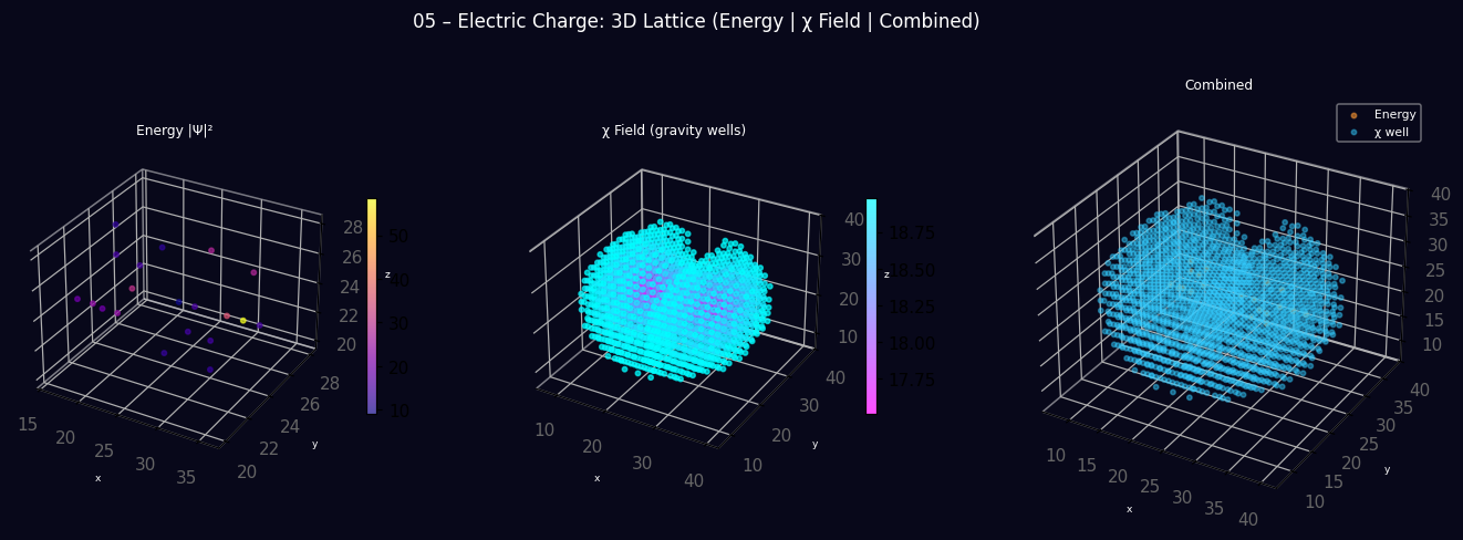
# ─── 3D Lattice Visualization ──────────────────────────────────────────────
# Requires matplotlib. Generates: tutorial_05_3d_lattice.png
# (Shows the opposite-phase pair after 3000 steps of attraction.)
try:
import matplotlib; matplotlib.use("Agg")
import matplotlib.pyplot as _plt
import numpy as _np
_N = sim_opp.chi.shape[0]
_step = max(1, _N // 20)
_idx = _np.arange(0, _N, _step)
_G = _np.meshgrid(_idx, _idx, _idx, indexing="ij")
_xx, _yy, _zz = _G[0].ravel(), _G[1].ravel(), _G[2].ravel()
_e = (sim_opp.psi_real[::_step, ::_step, ::_step] ** 2).ravel()
if sim_opp.psi_imag is not None:
_e = _e + (sim_opp.psi_imag[::_step, ::_step, ::_step] ** 2).ravel()
_ch = sim_opp.chi[::_step, ::_step, ::_step].ravel()
_bg = "#08081a"
_fig = _plt.figure(figsize=(15, 5), facecolor=_bg)
_fig.suptitle("05 – Electric Charge: 3D Lattice (Energy | χ Field | Combined)",
color="white", fontsize=11)
_chi_range = _ch.max() - _ch.min()
_chi_lo = _ch.max() - max(_chi_range * 0.05, 0.1)
for _col, (_ttl, _v, _cm, _lo) in enumerate([
("Energy |Ψ|²", _e, "plasma", max(_e.max() * 0.15, 1e-9)),
("χ Field (gravity wells)", _ch, "cool_r", _chi_lo),
]):
_ax = _fig.add_subplot(1, 3, _col + 1, projection="3d")
_ax.set_facecolor(_bg)
_mask = (_v < _lo) if _col == 1 else (_v > _lo)
if _mask.any():
_sc = _ax.scatter(_xx[_mask], _yy[_mask], _zz[_mask],
c=_v[_mask], cmap=_cm, s=8, alpha=0.70)
_plt.colorbar(_sc, ax=_ax, shrink=0.46, pad=0.07)
_ax.set_title(_ttl, color="white", fontsize=8)
for _t in (_ax.get_xticklabels() + _ax.get_yticklabels() +
_ax.get_zticklabels()):
_t.set_color("#666")
_ax.set_xlabel("x", color="w", fontsize=6)
_ax.set_ylabel("y", color="w", fontsize=6)
_ax.set_zlabel("z", color="w", fontsize=6)
_ax.xaxis.pane.fill = _ax.yaxis.pane.fill = _ax.zaxis.pane.fill = False
_ax.grid(color="gray", alpha=0.07)
_ax3 = _fig.add_subplot(1, 3, 3, projection="3d"); _ax3.set_facecolor(_bg)
_em = _e > _e.max() * 0.15 if _e.max() > 0 else _np.zeros_like(_e, dtype=bool)
_cm2 = _ch < _chi_lo
if _em.any(): _ax3.scatter(_xx[_em], _yy[_em], _zz[_em],
c="#ff9933", s=8, alpha=0.55, label="Energy")
if _cm2.any(): _ax3.scatter(_xx[_cm2], _yy[_cm2], _zz[_cm2],
c="#33ccff", s=8, alpha=0.45, label="χ well")
_ax3.legend(fontsize=7, labelcolor="white", facecolor=_bg, framealpha=0.5)
_ax3.set_title("Combined", color="white", fontsize=8)
for _t in (_ax3.get_xticklabels() + _ax3.get_yticklabels() +
_ax3.get_zticklabels()):
_t.set_color("#666")
_ax3.set_xlabel("x", color="w", fontsize=6)
_ax3.set_ylabel("y", color="w", fontsize=6)
_ax3.set_zlabel("z", color="w", fontsize=6)
_ax3.xaxis.pane.fill = _ax3.yaxis.pane.fill = _ax3.zaxis.pane.fill = False
_plt.tight_layout()
_plt.savefig("tutorial_05_3d_lattice.png", dpi=110, bbox_inches="tight",
facecolor=_bg)
_plt.close()
print()
print("Saved: tutorial_05_3d_lattice.png (3D: Energy | χ | Combined)")
except ImportError:
print()
print("(install matplotlib to generate 3D visualization)")Step-by-step explanation
Step 1 — Enable complex fields
config = lfm.SimulationConfig( grid_size=48, field_level=lfm.FieldLevel.COMPLEX, )FieldLevel.COMPLEX allocates both psi_real and psi_imag arrays. This is the minimum needed to represent U(1) phase, which is what electric charge is.
Step 2 — Set up two controlled experiments
# Same charge: both θ=0 sim_same.place_soliton(..., phase=0.0) sim_same.place_soliton(..., phase=0.0) # Opposite charge: θ=0 and θ=π sim_opp.place_soliton(..., phase=0.0) sim_opp.place_soliton(..., phase=np.pi)Running both systems from the same initial separation lets you directly compare the force — the only variable is the phase difference.
Step 3 — Compare separations after 3000 steps
Same phase (same charge) → separation increases slightly or stays flat (gravity and EM partially cancel). Opposite phase (opposite charge) → separation decreases faster than gravity alone. The difference is the electromagnetic signature.
Expected output
05 – Electric Charge
=======================================================

Same phase (both θ=0, same 'charge'):
  Initial separation: 14.0
  Final separation:   14.8
  Change: +0.8 cells

Opposite phase (θ=0 and θ=π, opposite 'charges'):
  Initial separation: 14.0
  Final separation:   10.9
  Change: -3.1 cells

Opposite charges attract MORE than same charges →
Coulomb-like behavior from pure wave interference!

Coulomb 1/r² scaling check (opposite-phase pairs):
    sep  Δsep/500 steps   1/r² (norm)
  -----  ---------------  ------------
     12            1.203         1.000
     16            0.671         0.563
     20            0.423         0.360

Closer pairs attract faster → ∝ 1/r²  (Coulomb without Coulomb's law).
No Coulomb's law was injected.  Charge = phase.
Visual preview
3D lattice produced by running the script above — |Ψ|² energy density, χ field, and combined view.