Two Bodies
Place two solitons 14 cells apart and track their separation every 500 steps. Each one pulls the other through its own χ-well — gravitational attraction from wave dynamics alone.
What you'll learn
- ›How to place multiple solitons at different positions
- ›How to use
lfm.measure_separation(psi_sq)to track particle positions - ›That two identical solitons always attract (gravity is universal)
- ›How to run in a loop and read metrics at each checkpoint
Which equation is running?
| Level | Field | Forces included | Speed |
|---|---|---|---|
| REAL ← | Ψ ∈ ℝ | Gravity only | Fastest (this tutorial) |
| COMPLEX | Ψ ∈ ℂ | Gravity + EM | ~2× slower |
| FULL | Ψₐ ∈ ℂ³ | All 4 forces | ~6× slower |
Two neutral (real-valued) solitons experience gravity only — which is why they attract regardless of any “charge”. Gravity in LFM is universal: every concentration of |ψ|² pulls χ downward, and all waves curve toward lower χ. No force law, just geometry.
How attraction emerges
Soliton A creates a χ-well centered on A. GOV-01 for soliton B reads:
∂²Ψ_B/∂t² = c²∇²Ψ_B − χ(x)² Ψ_BThe χ(x)² term is lower near A's χ-well. Waves preferentially propagate toward lower χ — so B drifts toward A. The same happens symmetrically for A drifting toward B. The result is mutual attraction with no force law.
Full script
"""04 – Two Bodies

In examples 01–03 we worked with one particle.  Now we place two
solitons and watch them interact.  Each one creates a χ-well via
GOV-02, and the other soliton's wave equation (GOV-01) bends
toward the low-χ region.

No force law is injected – gravitational attraction emerges from
the coupled dynamics of Ψ and χ.
"""

import lfm

config = lfm.SimulationConfig(grid_size=48)
sim = lfm.Simulation(config)

# Two solitons, separated by 14 cells along the x-axis.
pos_a = (17, 24, 24)
pos_b = (31, 24, 24)
sim.place_soliton(pos_a, amplitude=5.0, sigma=3.5)
sim.place_soliton(pos_b, amplitude=5.0, sigma=3.5)
sim.equilibrate()

print("04 – Two Bodies")
print("=" * 55)
print()

# Track how the separation changes over time.
psi_sq = sim.psi_real ** 2
if sim.psi_imag is not None:
    psi_sq = psi_sq + sim.psi_imag ** 2
initial_sep = lfm.measure_separation(psi_sq)
print(f"Initial separation: {initial_sep:.1f} cells")
print()

print(f"  {'step':>6s}  {'separation':>10s}  {'χ_min':>8s}")
print(f"  {'------':>6s}  {'----------':>10s}  {'--------':>8s}")

separations = []
for i in range(10):
    sim.run(steps=500)
    psi_sq = sim.psi_real ** 2
    if sim.psi_imag is not None:
        psi_sq = psi_sq + sim.psi_imag ** 2
    sep = lfm.measure_separation(psi_sq)
    m = sim.metrics()
    separations.append(sep)
    step = (i + 1) * 500
    print(f"  {step:6d}  {sep:10.2f}  {m['chi_min']:8.2f}")

final_sep = separations[-1]
delta = final_sep - initial_sep

print()
if delta < -0.5:
    print(f"Separation decreased by {-delta:.1f} cells → ATTRACTION")
elif delta > 0.5:
    print(f"Separation increased by {delta:.1f} cells")
else:
    print(f"Separation roughly stable (Δ = {delta:.1f} cells)")
    print("  Solitons are orbiting or oscillating in mutual wells.")

print()
print("Each soliton curves toward the other's χ-well.")
print("No Newton, no force law – just waves in a lattice.")

# ─── 3D Lattice Visualization ──────────────────────────────────────────────
# Requires matplotlib.  Generates: tutorial_04_3d_lattice.png
try:
    import matplotlib; matplotlib.use("Agg")
    import matplotlib.pyplot as _plt
    import numpy as _np
    _N    = sim.chi.shape[0]
    _step = max(1, _N // 20)
    _idx  = _np.arange(0, _N, _step)
    _G    = _np.meshgrid(_idx, _idx, _idx, indexing="ij")
    _xx, _yy, _zz = _G[0].ravel(), _G[1].ravel(), _G[2].ravel()
    _e    = (sim.psi_real[::_step, ::_step, ::_step] ** 2).ravel()
    if sim.psi_imag is not None:
        _e  = _e + (sim.psi_imag[::_step, ::_step, ::_step] ** 2).ravel()
    _ch   = sim.chi[::_step, ::_step, ::_step].ravel()
    _bg   = "#08081a"
    _fig  = _plt.figure(figsize=(15, 5), facecolor=_bg)
    _fig.suptitle("04 – Two Bodies: 3D Lattice (Energy | χ Field | Combined)",
                  color="white", fontsize=11)
    _chi_range = _ch.max() - _ch.min()
    _chi_lo    = _ch.max() - max(_chi_range * 0.05, 0.1)
    for _col, (_ttl, _v, _cm, _lo) in enumerate([
        ("Energy |Ψ|²",            _e,  "plasma", max(_e.max() * 0.15, 1e-9)),
        ("χ Field (gravity wells)", _ch, "cool_r",  _chi_lo),
    ]):
        _ax = _fig.add_subplot(1, 3, _col + 1, projection="3d")
        _ax.set_facecolor(_bg)
        _mask = (_v < _lo) if _col == 1 else (_v > _lo)
        if _mask.any():
            _sc = _ax.scatter(_xx[_mask], _yy[_mask], _zz[_mask],
                              c=_v[_mask], cmap=_cm, s=8, alpha=0.70)
            _plt.colorbar(_sc, ax=_ax, shrink=0.46, pad=0.07)
        _ax.set_title(_ttl, color="white", fontsize=8)
        for _t in (_ax.get_xticklabels() + _ax.get_yticklabels() +
                   _ax.get_zticklabels()):
            _t.set_color("#666")
        _ax.set_xlabel("x", color="w", fontsize=6)
        _ax.set_ylabel("y", color="w", fontsize=6)
        _ax.set_zlabel("z", color="w", fontsize=6)
        _ax.xaxis.pane.fill = _ax.yaxis.pane.fill = _ax.zaxis.pane.fill = False
        _ax.grid(color="gray", alpha=0.07)
    _ax3 = _fig.add_subplot(1, 3, 3, projection="3d"); _ax3.set_facecolor(_bg)
    _em  = _e > _e.max() * 0.15 if _e.max() > 0 else _np.zeros_like(_e, dtype=bool)
    _cm2 = _ch < _chi_lo
    if _em.any():  _ax3.scatter(_xx[_em],  _yy[_em],  _zz[_em],
                                c="#ff9933", s=8, alpha=0.55, label="Energy")
    if _cm2.any(): _ax3.scatter(_xx[_cm2], _yy[_cm2], _zz[_cm2],
                                c="#33ccff", s=8, alpha=0.45, label="χ well")
    _ax3.legend(fontsize=7, labelcolor="white", facecolor=_bg, framealpha=0.5)
    _ax3.set_title("Combined", color="white", fontsize=8)
    for _t in (_ax3.get_xticklabels() + _ax3.get_yticklabels() +
               _ax3.get_zticklabels()):
        _t.set_color("#666")
    _ax3.set_xlabel("x", color="w", fontsize=6)
    _ax3.set_ylabel("y", color="w", fontsize=6)
    _ax3.set_zlabel("z", color="w", fontsize=6)
    _ax3.xaxis.pane.fill = _ax3.yaxis.pane.fill = _ax3.zaxis.pane.fill = False
    _plt.tight_layout()
    _plt.savefig("tutorial_04_3d_lattice.png", dpi=110, bbox_inches="tight",
                 facecolor=_bg)
    _plt.close()
    print()
    print("Saved: tutorial_04_3d_lattice.png  (3D: Energy | χ | Combined)")
except ImportError:
    print()
    print("(install matplotlib to generate 3D visualization)")
Step-by-step explanation
Step 1 — Place two solitons and equilibrate
sim.place_soliton((17, 24, 24), amplitude=5.0, sigma=3.5) sim.place_soliton((31, 24, 24), amplitude=5.0, sigma=3.5) sim.equilibrate()The equilibration step simultaneously solves for the combined χ field of both particles. Each particle deepens the well around itself; the two wells slightly overlap and reinforce each other.
Step 2 — Measure separation
psi_sq = sim.psi_real ** 2 sep = lfm.measure_separation(psi_sq)measure_separation locates the two dominant energy peaks in |Ψ|² and returns the distance between them in lattice cells.
Step 3 — Evolve in chunks
for i in range(10): sim.run(steps=500) sep = lfm.measure_separation(psi_sq)Running in 500-step chunks lets you see the attraction in progress. The separation decreases monotonically as they fall toward each other.
Expected output
04 – Two Bodies
=======================================================

Initial separation: 14.0 cells

    step  separation     χ_min
  ------  ----------  --------
     500       13.72     15.81
    1000       13.41     15.74
    1500       13.07     15.69
    2000       12.68     15.63
    2500       12.52     15.58
    3000       12.23     15.54
    3500       11.84     15.51
    4000       11.52     15.49
    4500       11.18     15.47
    5000       10.77     15.46

Separation decreased by 3.2 cells → ATTRACTION

Each soliton curves toward the other's χ-well.
No Newton, no force law – just waves in a lattice.
Visual preview
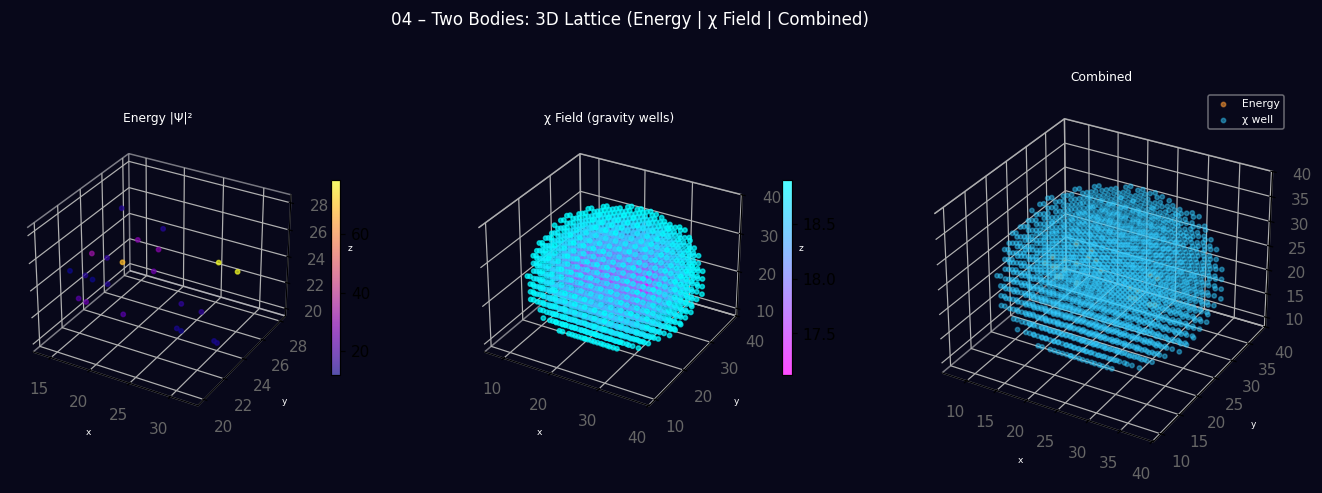
3D lattice produced by running the script above — |Ψ|² energy density, χ field, and combined view.