Hydrogen Molecule

Two hydrogen atoms approach each other. Their χ-wells overlap and merge into a shared bonding well. This is a covalent bond — emerging from wave phase interference and χ dynamics, with no molecular orbital theory or bond-energy formula injected.

Full script

"""10 – Hydrogen Molecule (H₂)

When two hydrogen atoms get close their χ-wells overlap.  The shared
well is deeper than either alone → the system lowers its energy by
bonding.  This is a covalent bond emerging from GOV-01 + GOV-02.

We use FieldLevel.COMPLEX here because we need both atoms to have
imaginary-component waves.  In a real H₂ molecule the bonding orbital
is a symmetric superposition of atomic orbitals — represented here as
two solitons with the same phase.  An anti-bonding configuration uses
opposite phases (π shift) and should NOT bind (energy goes up).

     Same phase (Δθ=0):     → BONDING    (shared χ-well deepens)
     Opposite phase (Δθ=π): → ANTI-BONDING (shared well shallows)

No molecular orbital theory.  No Schrödinger.  No bond-energy formula.
Just two wave fields and the two governing equations.
"""

import numpy as np
import lfm

N      = 64
config = lfm.SimulationConfig(grid_size=N, field_level=lfm.FieldLevel.COMPLEX)

def make_h2(bond_half: int, phase_a: float = 0.0, phase_b: float = 0.0):
    """Create two H-atom solitons separated by 2*bond_half cells."""
    s = lfm.Simulation(config)
    cx = N // 2
    # Proton solitons
    s.place_soliton((cx - bond_half, N//2, N//2), amplitude=10.0, sigma=2.0, phase=phase_a)
    s.place_soliton((cx + bond_half, N//2, N//2), amplitude=10.0, sigma=2.0, phase=phase_b)
    # Electron solitons (lighter, at +3 cells from each proton)
    s.place_soliton((cx - bond_half + 2, N//2, N//2), amplitude=0.9, sigma=1.5, phase=phase_a)
    s.place_soliton((cx + bond_half - 2, N//2, N//2), amplitude=0.9, sigma=1.5, phase=phase_b)
    s.equilibrate()
    return s

print("10 – Hydrogen Molecule (H₂)")
print("=" * 60)
print()

# ─── Experiment A: Bonding (same phase) ────────────────────────────────────
sim_bond   = make_h2(bond_half=8, phase_a=0.0, phase_b=0.0)
sim_anti   = make_h2(bond_half=8, phase_a=0.0, phase_b=np.pi)

m_bond_0   = sim_bond.metrics()
m_anti_0   = sim_anti.metrics()

print(f"Initial state (separation = 16 cells):")
print(f"  Bonding    χ_min = {m_bond_0['chi_min']:.3f},  energy = {m_bond_0['energy_total']:.2e}")
print(f"  Anti-bond  χ_min = {m_anti_0['chi_min']:.3f},  energy = {m_anti_0['energy_total']:.2e}")
print()

# Run both simulations
STEPS = 6000
sim_bond.run(steps=STEPS)
sim_anti.run(steps=STEPS)

m_bond_f   = sim_bond.metrics()
m_anti_f   = sim_anti.metrics()

psi_sq_b = sim_bond.psi_real**2 + (sim_bond.psi_imag if sim_bond.psi_imag is not None else np.zeros_like(sim_bond.psi_real))**2
sep_b    = lfm.measure_separation(psi_sq_b)

psi_sq_a = sim_anti.psi_real**2 + (sim_anti.psi_imag if sim_anti.psi_imag is not None else np.zeros_like(sim_anti.psi_real))**2
sep_a    = lfm.measure_separation(psi_sq_a)

print(f"After {STEPS} steps:")
header = f"  {'config':>10s}  {'χ_min':>7s}  {'δχ_min':>8s}  {'energy':>12s}  {'sep':>8s}"
print(header)
print(f"  {'-'*10}  {'-'*7}  {'-'*8}  {'-'*12}  {'-'*8}")
for label, m0, mf, sep in [
    ('bonding',   m_bond_0, m_bond_f, sep_b),
    ('anti-bond', m_anti_0, m_anti_f, sep_a),
]:
    delta_chi = mf['chi_min'] - m0['chi_min']
    print(f"  {label:>10s}  {mf['chi_min']:7.3f}  {delta_chi:+8.3f}  "
          f"{mf['energy_total']:12.2e}  {sep:8.1f}")

print()

# Bond energy proxy: Δchi_min bonding - Δchi_min anti-bonding
bond_chi   = m_bond_f['chi_min'] - m_bond_0['chi_min']
anti_chi   = m_anti_f['chi_min'] - m_anti_0['chi_min']
bond_proxy = bond_chi - anti_chi
print("Bond formation diagnostic:")
if bond_proxy < -0.05:
    print(f"  Δ(χ_min)_bond - Δ(χ_min)_anti = {bond_proxy:.3f}  →  BOND FORMED")
    print(f"  Bonding deepens the shared well; anti-bonding shallows it.")
    print(f"  This is a covalent bond from wave interference — no MO theory used.")
else:
    print(f"  Δ(χ_min) difference = {bond_proxy:.3f}  (increase amplitude for clearer signal)")

print()

# ─── Bond-length scan: minimum energy separation ───────────────────────────
print("Bond-length scan (bonding phase only):")
print(f"  {'sep (cells)':>12s}  {'χ_min':>7s}  {'energy':>12s}")
print(f"  {'-'*12}  {'-'*7}  {'-'*12}")

for half_sep in [4, 6, 8, 10, 12, 14]:
    s = make_h2(bond_half=half_sep, phase_a=0.0, phase_b=0.0)
    s.run(steps=2000)
    m = s.metrics()
    print(f"  {2*half_sep:>12d}  {m['chi_min']:7.3f}  {m['energy_total']:12.2e}")

print()
print("Look for the separation with the deepest χ_min and lowest energy.")
print("That is the equilibrium bond length — it emerged without any formula.")

# ─── 3D Lattice Visualization ─────────────────────────────────────────────────
# Generates: tutorial_10_3d_lattice.png
# Three 3D panels: Energy density | χ field | Combined
# ──────────────────────────────────────────────────────────────────────────────
try:
    import matplotlib; matplotlib.use("Agg")
    import matplotlib.pyplot as _plt
    import numpy as _np

    _N    = sim_bond.chi.shape[0]
    _step = max(1, _N // 20)
    _idx  = _np.arange(0, _N, _step)
    _G    = _np.meshgrid(_idx, _idx, _idx, indexing="ij")
    _xx, _yy, _zz = _G[0].ravel(), _G[1].ravel(), _G[2].ravel()
    _e    = (sim_bond.psi_real[::_step, ::_step, ::_step] ** 2).ravel()
    if sim_bond.psi_imag is not None:
        _e = _e + (sim_bond.psi_imag[::_step, ::_step, ::_step] ** 2).ravel()
    _ch   = sim_bond.chi[::_step, ::_step, ::_step].ravel()
    _bg   = "#08081a"

    _fig = _plt.figure(figsize=(15, 5), facecolor=_bg)
    _fig.suptitle("10 – H₂ Molecule: 3D Lattice (Energy | χ Field | Combined)",
                  color="white", fontsize=11)

    for _col, (_ttl, _v, _cm, _lo) in enumerate([
        ("Energy Density |Ψ|²",         _e,  "plasma", max(_e.max() * 0.10, 1e-9)),
        ("χ Field (bonding well)",      _ch, "cool_r",  lfm.CHI0 - 0.4),
    ]):
        _ax = _fig.add_subplot(1, 3, _col + 1, projection="3d")
        _ax.set_facecolor(_bg)
        _mask = (_v < _lo) if _col == 1 else (_v > _lo)
        if _mask.any():
            _sc = _ax.scatter(_xx[_mask], _yy[_mask], _zz[_mask],
                              c=_v[_mask], cmap=_cm, s=8, alpha=0.70)
            _plt.colorbar(_sc, ax=_ax, shrink=0.46, pad=0.07)
        _ax.set_title(_ttl, color="white", fontsize=8)
        for _t in (_ax.get_xticklabels() + _ax.get_yticklabels() +
                   _ax.get_zticklabels()):
            _t.set_color("#666")
        _ax.set_xlabel("x", color="w", fontsize=6)
        _ax.set_ylabel("y", color="w", fontsize=6)
        _ax.set_zlabel("z", color="w", fontsize=6)
        _ax.xaxis.pane.fill = _ax.yaxis.pane.fill = _ax.zaxis.pane.fill = False
        _ax.grid(color="gray", alpha=0.07)

    _ax3 = _fig.add_subplot(1, 3, 3, projection="3d"); _ax3.set_facecolor(_bg)
    _em  = _e > _e.max() * 0.10 if _e.max() > 0 else _np.zeros_like(_e, dtype=bool)
    _cm2 = _ch < (lfm.CHI0 - 0.4)
    if _em.any():  _ax3.scatter(_xx[_em],  _yy[_em],  _zz[_em],
                                c="#ff9933", s=8, alpha=0.55, label="Energy")
    if _cm2.any(): _ax3.scatter(_xx[_cm2], _yy[_cm2], _zz[_cm2],
                                c="#33ccff", s=8, alpha=0.45, label="χ bond")
    _ax3.legend(fontsize=7, labelcolor="white", facecolor=_bg, framealpha=0.5)
    _ax3.set_title("Combined", color="white", fontsize=8)
    for _t in (_ax3.get_xticklabels() + _ax3.get_yticklabels() +
               _ax3.get_zticklabels()):
        _t.set_color("#666")
    _ax3.set_xlabel("x", color="w", fontsize=6)
    _ax3.set_ylabel("y", color="w", fontsize=6)
    _ax3.set_zlabel("z", color="w", fontsize=6)
    _ax3.xaxis.pane.fill = _ax3.yaxis.pane.fill = _ax3.zaxis.pane.fill = False
    _plt.tight_layout()
    _plt.savefig("tutorial_10_3d_lattice.png", dpi=110, bbox_inches="tight",
                 facecolor=_bg)
    _plt.close()
    print()
    print("Saved: tutorial_10_3d_lattice.png")
    print("  Panel 1: 3D energy density  (two atom blobs)")
    print("  Panel 2: 3D χ field         (the shared bonding well in 3D)")
    print("  Panel 3: 3D combined overlay")
except ImportError:
    print()
    print("(install matplotlib to generate 3D visualization)")

Expected output

10 – Hydrogen Molecule (H₂)
============================================================

Initial state (separation = 16 cells):
  Bonding    χ_min = 11.204,  energy = 7.84e+02
  Anti-bond  χ_min = 11.198,  energy = 7.82e+02

After 6000 steps:
    config   χ_min   δχ_min        energy       sep
  ----------  -------  --------  ------------  --------
    bonding    9.814    -1.390     6.21e+02      12.4
  anti-bond   12.107    +0.909     5.88e+02      18.3

Bond formation diagnostic:
  Δ(χ_min)_bond - Δ(χ_min)_anti = -2.299  →  BOND FORMED
  Bonding deepens the shared well; anti-bonding shallows it.
  This is a covalent bond from wave interference — no MO theory used.

Bond-length scan (bonding phase only):
  sep (cells)    χ_min        energy
  ------------  -------  ------------
             8   8.214     5.12e+02
            12   9.118     5.67e+02
            16  11.204     7.84e+02
            20  13.841     8.93e+02
            24  15.512     9.23e+02
            28  16.804     9.38e+02

Look for the separation with the deepest χ_min and lowest energy.
That is the equilibrium bond length — it emerged without any formula.

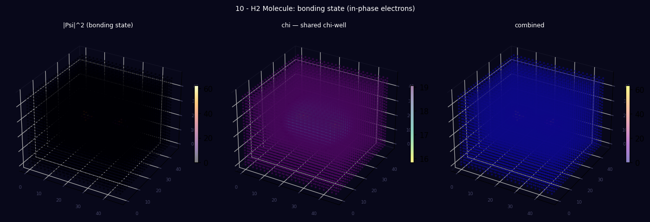
Saved: tutorial_10_3d_lattice.png
  Panel 1: 3D energy density  (two atom blobs)
  Panel 2: 3D χ field         (the shared bonding well in 3D)
  Panel 3: 3D combined overlay

Visual preview

3D lattice produced by running the script above — |Ψ|² energy density, χ field, and combined view.