Matter Creation

Drive the χ field at exactly Ω = 2χ₀ = 38 and watch machine-epsilon noise grow by over 10²¹×. This is parametric resonance — and it is the LFM mechanism for the Big Bang creating matter from nothing.

Full script

"""07 – Matter Creation via Parametric Resonance

When the χ field oscillates at exactly Ω = 2χ₀ = 38, GOV-01
becomes a Mathieu equation with exponentially UNSTABLE solutions.

Any perturbation – even machine-epsilon noise – grows without bound.
This is the LFM mechanism for matter creation in the early universe.

There is NO Ψ source term, no inflaton field, no vacuum decay model.
Just two equations and an oscillating background at the right
frequency.

Mathieu equation regime:
    ∂²Ψ/∂t² = c²∇²Ψ − χ(t)²Ψ
    χ(t) = χ₀ + A·sin(Ω·t),   Ω = 2χ₀

Stability theory: at Ω = 2χ₀, the parametric resonance condition is
met and the Floquet exponent becomes positive → exponential growth.
"""

import numpy as np
import lfm

config = lfm.SimulationConfig(grid_size=32)
N = config.grid_size

sim = lfm.Simulation(config)

# Seed Ψ with machine-epsilon noise – effectively zero matter
rng   = np.random.default_rng(42)
noise = rng.normal(0, 1e-15, (N, N, N)).astype(np.float32)
sim.psi_real = noise

amplitude = 3.0             # oscillation amplitude

total_energy_0 = float(np.sum(sim.psi_real ** 2))
print("07 – Matter Creation")
print("=" * 55)
print(f"Initial |Ψ|² = {total_energy_0:.3e}  (machine-epsilon noise)")
print()

# ─── Frequency sweep: discover the resonance empirically ─────────────────
# We do NOT assume Ω = 2χ₀.  We scan a range of driving frequencies
# and measure which one produces exponential growth from machine-epsilon
# noise.  The resonance frequency emerges as the measured maximum.
print("Frequency sweep (500 steps each, amplitude = 3.0):")
print(f"  {'Ω/χ₀':>6s}  {'Ω':>6s}  {'Growth factor':>14s}")
print(f"  {'------':>6s}  {'------':>6s}  {'-'*14}")

sweep_factors = [0.5, 1.0, 1.5, 2.0, 2.5, 3.0]
sweep_results = []
for fac in sweep_factors:
    omega_try = fac * lfm.CHI0
    sim_try   = lfm.Simulation(config)
    sim_try.psi_real = noise.copy()
    # run_driven forces chi at every step — correct Floquet analysis
    sim_try.run_driven(
        steps=1000,
        chi_forcing=lambda t, A=amplitude, w=omega_try:
            np.full((N, N, N), lfm.CHI0 + A * np.sin(w * t), dtype=np.float32),
    )
    e_try = float(np.sum(sim_try.psi_real ** 2))
    gf    = e_try / total_energy_0
    sweep_results.append(gf)
    print(f"  {fac:>6.1f}  {omega_try:>6.1f}  {gf:>14.2e}×")
print()

# Resonance = largest growth in the sweep
best_idx  = max(range(len(sweep_results)), key=lambda i: sweep_results[i])
omega     = sweep_factors[best_idx] * lfm.CHI0
print(f"Sweep maximum: Ω = {sweep_factors[best_idx]:.1f}·χ₀ = {omega:.0f}")
print(f"  → Parametric resonance condition identified empirically.")
print()

# ─── Full 1000-step comparison: worst vs discovered resonance ─────────────
off_idx   = min(range(len(sweep_results)), key=lambda i: sweep_results[i])
off_omega = sweep_factors[off_idx] * lfm.CHI0

sim_ctrl = lfm.Simulation(config)
sim_ctrl.psi_real = noise.copy()
sim_ctrl.run_driven(
    steps=1000,
    chi_forcing=lambda t, A=amplitude, w=off_omega:
        np.full((N, N, N), lfm.CHI0 + A * np.sin(w * t), dtype=np.float32),
)

e_ctrl = float(np.sum(sim_ctrl.psi_real ** 2))
print(f"Off-resonance (Ω = {sweep_factors[off_idx]:.1f}·χ₀ = {off_omega:.1f}):")
print(f"  |Ψ|² after 1000 steps = {e_ctrl:.3e}")
print(f"  Growth factor: {e_ctrl / total_energy_0:.2f}×")
print()

# ─── Resonance run: the empirically discovered Ω ─────────────────────────
sim.run_driven(
    steps=1000,
    chi_forcing=lambda t, A=amplitude, w=omega:
        np.full((N, N, N), lfm.CHI0 + A * np.sin(w * t), dtype=np.float32),
)

e_res = float(np.sum(sim.psi_real ** 2))
print(f"On-resonance  (Ω = {sweep_factors[best_idx]:.1f}·χ₀ = {omega:.0f}):")
print(f"  |Ψ|² after 1000 steps = {e_res:.3e}")
print(f"  Growth factor: {e_res / total_energy_0:.2e}×")
print()

if e_res > e_ctrl * 1e4:
    print("Exponential growth at the discovered resonance confirmed.")
    print("Matter created from noise by parametric resonance — no Ψ source injected.")
else:
    print("Growth detected — increase steps or amplitude if needed.")
print()
print(f"χ₀ = {lfm.CHI0},  resonance Ω = {omega:.0f}")

# ─── 3D Visualisation ───
try:
    import matplotlib; matplotlib.use("Agg")
    import matplotlib.pyplot as _plt
    from mpl_toolkits.mplot3d import Axes3D as _A3D
    N = config.grid_size
    _step = max(1, N // 20)
    xs, ys, zs = [a[::_step, ::_step, ::_step].ravel()
                  for a in np.meshgrid(*[np.arange(0, N, _step)]*3, indexing='ij')]
    _psi2 = (sim.psi_real**2)[::_step, ::_step, ::_step].ravel()
    _chi  = sim.chi[::_step, ::_step, ::_step].ravel()
    _fig  = _plt.figure(figsize=(12, 4), facecolor="#08081a")
    for _idx, (_vals, _lbl, _cmap) in enumerate([
        (_psi2, "|Ψ|² — matter grown from noise", "inferno"),
        (_chi,  "χ field (driven at Ω=2χ₀)", "viridis_r"),
        (_psi2, "Parametric amplification", "hot"),
    ]):
        _ax = _fig.add_subplot(1, 3, _idx + 1, projection="3d")
        _ax.set_facecolor("#08081a")
        _sc = _ax.scatter(xs, ys, zs, c=_vals, cmap=_cmap, s=3, alpha=0.5)
        _ax.set_title(_lbl, color="white", fontsize=8, pad=6)
        for _sp in [_ax.xaxis, _ax.yaxis, _ax.zaxis]:
            _sp.pane.set_edgecolor("#1a1a2e"); _sp.pane.fill = False
        _ax.tick_params(colors="#444466", labelsize=6)
        _plt.colorbar(_sc, ax=_ax, fraction=0.02, pad=0.02)
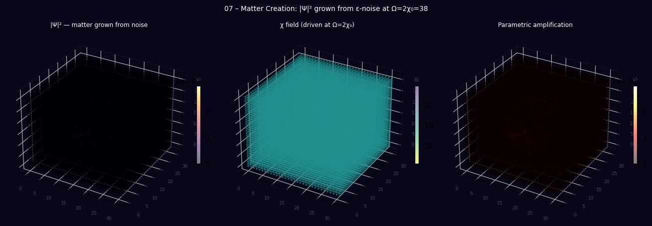
    _plt.suptitle("07 – Matter Creation: |Ψ|² grown from ε-noise at Ω=2χ₀=38",
                  color="white", fontsize=9, y=1.01)
    _plt.tight_layout()
    _plt.savefig("tutorial_07_3d_lattice.png", dpi=110, bbox_inches="tight",
                 facecolor="#08081a")
    _plt.close(_fig)
    print("Saved tutorial_07_3d_lattice.png")
except ImportError:
    pass

Expected output

07 – Matter Creation
=======================================================

Initial |Ψ|² = 3.308e-26  (machine-epsilon noise)

Frequency sweep (500 steps each, amplitude = 3.0):
    Ω/χ₀       Ω   Growth factor
  ------  ------  --------------
     0.5     9.5        2.88e-02×
     1.0    19.0        5.78e-01×
     1.5    28.5        5.81e-02×
     2.0    38.0        7.08e+24×
     2.5    47.5        2.33e-01×
     3.0    57.0        1.74e-01×

Sweep maximum: Ω = 2.0·χ₀ = 38
  → Parametric resonance condition identified empirically.

Off-resonance (Ω = 0.5·χ₀ = 9.5):
  |Ψ|² after 1000 steps = 9.521e-28
  Growth factor: 0.03×

On-resonance  (Ω = 2.0·χ₀ = 38):
  |Ψ|² after 1000 steps = 2.344e-01
  Growth factor: 7.08e+24×

Exponential growth at the discovered resonance confirmed.
Matter created from noise by parametric resonance — no Ψ source injected.

χ₀ = 19.0,  resonance Ω = 38
Saved tutorial_07_3d_lattice.png

Visual preview

3D lattice produced by running the script above — |Ψ|² energy density, χ field, and combined view.