Your First Particle
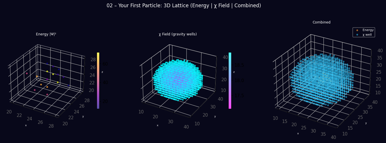
Place a blob of energy on the lattice. GOV-02 responds by pullingχbelow 19 — creating a gravitational well. No Newton's law is added.
What you'll learn
- ›How to place a soliton with
sim.place_soliton(center, amplitude, sigma) - ›Why you must call
sim.equilibrate()before evolving - ›How to interpret
chi_minas gravitational well depth - ›That gravity emerges from GOV-02, not from Newton's law
Which equation is running?
| Level | Field | Forces included | Speed |
|---|---|---|---|
| REAL ← | Ψ ∈ ℝ | Gravity only | Fastest (this tutorial) |
| COMPLEX | Ψ ∈ ℂ | Gravity + EM | ~2× slower |
| FULL | Ψₐ ∈ ℂ³ | All 4 forces | ~6× slower |
FULL is always physically correct — it is simply slower. This tutorial uses REAL because we are studying gravity only and real fields are 6× faster. Gravity in LFM comes entirely from the |ψ|² term in GOV-02, which behaves identically for real and complex fields.
The Key idea: GOV-02
GOV-02 is the equation that governs χ:
∂²χ/∂t² = c²∇²χ − κ(|Ψ|² − E₀²)Where there is a concentration of wave energy |Ψ|², GOV-02 drives χ downward. Low χ means a stiffer medium with a deeper potential well — waves curve toward it. That curvature is gravity.
Full script
"""02 – Your First Particle

Drop a lump of energy onto the lattice and watch gravity appear.

In example 01 we saw that empty space has χ = 19 everywhere.
Now we add energy: a Gaussian soliton (a smooth blob of wave
amplitude).  GOV-02 says that energy density |Ψ|² pulls χ
downward.  Low χ = gravitational well.

This is gravity emerging from nothing but the wave equations.
"""

import lfm

config = lfm.SimulationConfig(grid_size=48)
sim = lfm.Simulation(config)

print("02 – Your First Particle")
print("=" * 55)
print()

# Place one soliton at the grid center.
center = (24, 24, 24)
sim.place_soliton(center, amplitude=5.0, sigma=4.0)

print("Before equilibration:")
m = sim.metrics()
print(f"  χ_min  = {m['chi_min']:.2f}  (should be 19 – no well yet)")
print()

# Equilibrate: solve Poisson equation so chi adjusts to the energy.
sim.equilibrate()

print("After equilibration (GOV-02 created the well):")
m = sim.metrics()
print(f"  χ_min  = {m['chi_min']:.2f}  (below 19 → gravity well!)")
print(f"  wells  = {m['well_fraction']*100:.1f}%  of the grid is a well")
print()

# Evolve – the soliton sits in its own gravity well.
sim.run(steps=2000)
m = sim.metrics()
print(f"After 2000 steps of evolution:")
print(f"  χ_min  = {m['chi_min']:.2f}")
print(f"  wells  = {m['well_fraction']*100:.1f}%")
print(f"  energy = {m['energy_total']:.2e}")
print()
print("The energy blob created a χ-well and sits inside it.")
print("No Newton's law was injected – gravity emerged from GOV-02.")
print()
print("Next: measure the shape of this well (→ 03).")

# ─── 3D Lattice Visualization ──────────────────────────────────────────────
# Requires matplotlib.  Generates: tutorial_02_3d_lattice.png
try:
    import matplotlib; matplotlib.use("Agg")
    import matplotlib.pyplot as _plt
    import numpy as _np
    _N    = sim.chi.shape[0]
    _step = max(1, _N // 20)
    _idx  = _np.arange(0, _N, _step)
    _G    = _np.meshgrid(_idx, _idx, _idx, indexing="ij")
    _xx, _yy, _zz = _G[0].ravel(), _G[1].ravel(), _G[2].ravel()
    _e    = (sim.psi_real[::_step, ::_step, ::_step] ** 2).ravel()
    if sim.psi_imag is not None:
        _e  = _e + (sim.psi_imag[::_step, ::_step, ::_step] ** 2).ravel()
    _ch   = sim.chi[::_step, ::_step, ::_step].ravel()
    _bg   = "#08081a"
    _fig  = _plt.figure(figsize=(15, 5), facecolor=_bg)
    _fig.suptitle("02 – Your First Particle: 3D Lattice (Energy | χ Field | Combined)",
                  color="white", fontsize=11)
    _chi_range = _ch.max() - _ch.min()
    _chi_lo    = _ch.max() - max(_chi_range * 0.05, 0.1)
    for _col, (_ttl, _v, _cm, _lo) in enumerate([
        ("Energy |Ψ|²",            _e,  "plasma", max(_e.max() * 0.15, 1e-9)),
        ("χ Field (gravity wells)", _ch, "cool_r",  _chi_lo),
    ]):
        _ax = _fig.add_subplot(1, 3, _col + 1, projection="3d")
        _ax.set_facecolor(_bg)
        _mask = (_v < _lo) if _col == 1 else (_v > _lo)
        if _mask.any():
            _sc = _ax.scatter(_xx[_mask], _yy[_mask], _zz[_mask],
                              c=_v[_mask], cmap=_cm, s=8, alpha=0.70)
            _plt.colorbar(_sc, ax=_ax, shrink=0.46, pad=0.07)
        _ax.set_title(_ttl, color="white", fontsize=8)
        for _t in (_ax.get_xticklabels() + _ax.get_yticklabels() +
                   _ax.get_zticklabels()):
            _t.set_color("#666")
        _ax.set_xlabel("x", color="w", fontsize=6)
        _ax.set_ylabel("y", color="w", fontsize=6)
        _ax.set_zlabel("z", color="w", fontsize=6)
        _ax.xaxis.pane.fill = _ax.yaxis.pane.fill = _ax.zaxis.pane.fill = False
        _ax.grid(color="gray", alpha=0.07)
    _ax3 = _fig.add_subplot(1, 3, 3, projection="3d"); _ax3.set_facecolor(_bg)
    _em  = _e > _e.max() * 0.15 if _e.max() > 0 else _np.zeros_like(_e, dtype=bool)
    _cm2 = _ch < _chi_lo
    if _em.any():  _ax3.scatter(_xx[_em],  _yy[_em],  _zz[_em],
                                c="#ff9933", s=8, alpha=0.55, label="Energy")
    if _cm2.any(): _ax3.scatter(_xx[_cm2], _yy[_cm2], _zz[_cm2],
                                c="#33ccff", s=8, alpha=0.45, label="χ well")
    _ax3.legend(fontsize=7, labelcolor="white", facecolor=_bg, framealpha=0.5)
    _ax3.set_title("Combined", color="white", fontsize=8)
    for _t in (_ax3.get_xticklabels() + _ax3.get_yticklabels() +
               _ax3.get_zticklabels()):
        _t.set_color("#666")
    _ax3.set_xlabel("x", color="w", fontsize=6)
    _ax3.set_ylabel("y", color="w", fontsize=6)
    _ax3.set_zlabel("z", color="w", fontsize=6)
    _ax3.xaxis.pane.fill = _ax3.yaxis.pane.fill = _ax3.zaxis.pane.fill = False
    _plt.tight_layout()
    _plt.savefig("tutorial_02_3d_lattice.png", dpi=110, bbox_inches="tight",
                 facecolor=_bg)
    _plt.close()
    print()
    print("Saved: tutorial_02_3d_lattice.png  (3D: Energy | χ | Combined)")
except ImportError:
    print()
    print("(install matplotlib to generate 3D visualization)")
Step-by-step explanation
Step 1 — Place the soliton
sim.place_soliton(center, amplitude=5.0, sigma=4.0)This writes a Gaussian blob — amplitude × exp(−r²/2σ²) — into the Ψ field. At this point χ is still flat at 19 everywhere; the energy is just sitting there with no well yet.
Step 2 — Equilibrate
sim.equilibrate()Solves the quasi-static Poisson equation (GOV-04) via FFT to find the χ profile that is consistent with the current energy distribution. After this, χ_min drops noticeably below 19.
Step 3 — Evolve and observe stability
sim.run(steps=2000) m = sim.metrics() print(m['chi_min'], m['wells'])The soliton sits in its own χ-well and remains bound. The well depth stays roughly constant — the particle has found a stable, self-consistent configuration.
Expected output
02 – Your First Particle
=======================================================

Before equilibration:
  χ_min  = 19.00  (should be 19 – no well yet)

After equilibration (GOV-02 created the well):
  χ_min  = 16.43  (below 19 → gravity well!)
  wells  = 2.3%  of the grid is a well

After 2000 steps of evolution:
  χ_min  = 16.38
  wells  = 2.4%
  energy = 3.21e+03

The energy blob created a χ-well and sits inside it.
No Newton's law was injected – gravity emerged from GOV-02.

Next: measure the shape of this well (→ 03).
Visual preview
3D lattice produced by running the script above — |Ψ|² energy density, χ field, and combined view.